Multi-domain Modeling in Ads
Contents
Background
In the field of recommendation system and digital ads, more and more companies are seeking to use a big model to serve all different businesses and channels (referred to as domains). This will not only reduce the cost of maintaining dozens of models, one for each domain, but also help enhance the ability of generalization of the prediction model by merging the enormous data into one single pool. However, the distributions of user features from these domains differ a lot. For example, the customers from a fashion e-commerce website and a mountain bike website may have few interests in common. To tackle this, we have to force the model to see the pattern behind each domain by explicitly feeding the domain identifiers into the model, such as the business id or the url of a website. But how do we make full use of this domain-related feature?
Note that the concept of multi-domain learning is totally different from domain adaptation, where the knowledge is transferred one-way from the source domain to the target domain.
Star Topology Adaptive Recommender (STAR)
Intro
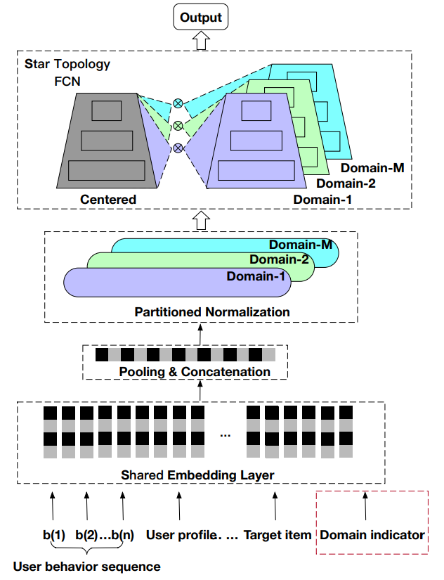
STAR proposes two crucial modules to solve the problem of multi-domain learning: Partitioned Normalization (PN) and Star Topology Fully-Connected Networks (FCN). The following picture shows the structure of STAR.

First, the embedding layer is shared across all domains. This is desirable since these embeddings take up most of storage. Then the embeddings are pooled and concatenated into one long vector. In the next step, PN is applied to the input vector and generates multiple representations for various domains. For the last stage, there will be two types of FCN, the shared FCN and the domain-specific FCNs.
Partitioned Normalization
Since the statistics of the features from different domains are inconsistent, we would like to normalize them with different parameters. Also, recall that for Batch Normalization, we assume the data inside a mini-batch to be identical and independent. Therefore, this paper proposes to use domain-specific scale and bias parameters to handle the gaps between distributions. Formally,
$$ \mathbf{z}^{\prime}=\left(\gamma * \gamma_{p}\right) \frac{\mathbf{z}-E_{p}}{\sqrt{\operatorname{Var}_{p}+\epsilon}}+\left(\beta+\beta_{p}\right) $$ where $p$ is the domain id, $\gamma, \beta$ are the global scale and bias parameters and $\gamma_p$ and $\beta_p$ are domain-specific scale and bias. And $E_p$ and $Var_p$ are the moving average of mean and variance of data from domain $p$.
Star Topology FCN

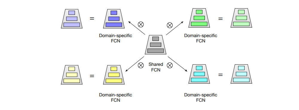
Similar to the idea of PN, there will be a shared FCN representing the common part of these domains and multiple domain-specific FCN learning the bias of each domain. You can see the origin of the name star topology from the picture above. For each domain, the weight $W^*_p$ is the product of the weights of the shared FCN and the FCN belonging to domain $p$, and the bias term is the sum of the two biases.
$$ W^*_p = W_p \otimes W, b^*_p = b_p + b $$
Hence, the output of Star Topology FCN associated with domain $p$ is
$$ {out}_p = \phi ((W_p^*)^T\ {in}_p + b^*_p) $$
AdaSparse
Basic Idea

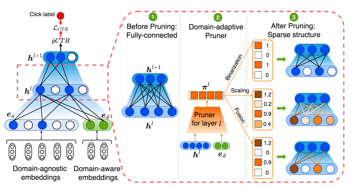
This paper also solves the problem of multi-domain learning in CTR prediction, but puts an emphasis on learning a sparse network to further improve the generalization ability and computational efficiency of the big model. Instead of multiplying weights of two FCNs, AdaSparse multiplies the output of each intermediate layer $\boldsymbol h^l$ with the output of a pruner sub-network $\boldsymbol \pi^l_d$. The pruners take the $\boldsymbol h^l$ and domain-aware embeddings $\boldsymbol e_d$ as input and predict the importance of each neuron. Thus, the multiplication can be seen as a process of dynamic pruning, or feature selection.
$$ \boldsymbol h^l_d = \boldsymbol h^l \odot \boldsymbol \pi^l_d $$
As shown in the figure above, there are three methods of generating $\boldsymbol \pi ^l$.
- Binarization: hard-thresholding the output to be 0 or 1.
$$S_{\epsilon}(v)=\operatorname{sign}\left(\left|\sigma\left(\alpha \cdot v\right)\right|-\epsilon\right)$$
where $\epsilon$ is a predefined small value and $\alpha$ is a continuously growing value.
- Scaling: a soft thresholding method, making important neurons have larger values. ($\beta \ge 1$)
$$S_{\epsilon}(v)=\beta\cdot \sigma (v) \operatorname{sign}(|\beta\cdot \sigma (v)|)$$
- Fusion: combine the two methods above, amplifying large values and forcing small values to 0.
$$S_{\epsilon}(v)=\beta\cdot \sigma (\alpha v) \operatorname{sign}(|\beta\cdot \sigma (\alpha v)| - \epsilon)$$
Learning a Sparse Structure
In machine learning, we know $\mathcal L_1$ regularization is the usual choice to get a sparse solution. The paper defines the sparsity ratio as $r^l = 1 - \frac{| \boldsymbol \pi^l |_1}{N^l}$ where $N^l$ is the dimension of $\boldsymbol \pi^l$. The authors hopes to explicitly control the sparsity of the model by forcing the $r^l$ to lie between $r_{min}$ and $r_{max}$. Therefore, the regularization term becomes:
$$
R_{s}=\frac{1}{L} \sum_{l=1}^{L} \lambda^{l} |r^{l}-r |_{2}, \quad r=(r_{\min }+r_{\max }) / 2 \
$$
$$\lambda^{l}=\begin{cases} 0 & r^{l} \in\left[r_{\min }, r_{\max }\right] \\ \hat{\lambda} \cdot\left|r^{l}-r\right| \quad & r^{l} \notin\left[r_{\min }, r_{\max }\right] \ \end{cases}$$
where $\hat \lambda$ is initialized by 0.01 and gradually increase over training step, thus the model pays less attention on sparsity loss term during early training and focuses more on adjusting $\boldsymbol \pi ^l$.