A Survey on Rule Learning in Text Mining
Contents
1. A Short Introduction to Probabilistic Soft Logic
Semantics
Rule: Body $\rightarrow$ Head $r = r_{body} \rightarrow r_{head} = \neg r_{body} \lor r_{head}$
Interpretation: A mapping $I: \ell \rightarrow [0,1]^{n}$, which provides a set of assignments to atoms, whose probabilities can then be determined. In mathematical logic, an assignment is mapping entities from domain $D$ to variables in a proposition and by assignment we get a boolean value of the proposition. A grouding of a rule represents an instantiation of all variables in the rule after assignment.
Given interpretation $I$, the logical operators are defined:
$$
\begin{aligned}
\ell_{1} \tilde{\wedge} \ell_{2}&=\max \left\{0, I\left(\ell_{1}\right)+I\left(\ell_{2}\right)-1\right\} \\
\ell_{1} \tilde{\vee} \ell_{2}&=\min \left\{I\left(\ell_{1}\right)+I\left(\ell_{2}\right), 1\right\} \\
\tilde\neg l_{1}&=1-I\left(\ell_{1}\right)
\end{aligned}
$$
then, probabilities of every rule can be calculated corresponding to the interpretation given.
Given $I$, for each rule we define a distance to satisfaction $$ d_r(I) = 1 - I(r) = \max{0, I(r_{body}) - I(r_{head})} $$
The probability is defined as: $$ f(I)=\frac{1}{Z} \exp \left[-\sum_{r \in R} \lambda_{r}\left(d_{r}(I)\right)^{p}\right] \quad ; \quad Z=\int_{I} \exp \left[-\sum_{r \in R} \lambda_{r}\left(d_{r}(I)\right)^{p}\right] $$ $p=1,2$, and $p=1$ favors strict satisfaction.
When $I$ violates any hard constraint (background knowledge), set $f(I)=0$
Inference & Learning
- Given interpretation of some propositions as evidence, find the most likely interpretation for the rest.
- Computie marginal distributions
The space of interpretations with non-zero density forms a convex polytope.
MPE Inference Optimization method: Second-Order Cone Program (SOCP) or consensus optimization
Computing Marginal Distributions For an atom $l_i$, computing $P(l\leq I(l_i)\leq u)$ corresponds to computing the volume of a slice of the convex polytope of non-zero density interpretations. Use hit-and-run Markov chain Monte Carlo to sample points in polytope and approximate the distribution.
Weight Learning $$ \frac{\partial}{\partial \lambda_{i}} \log f(I)=-\sum_{r \in R_{i}}\left(d_{r}(I)\right)^{p}+\mathbb{E}\left[\sum_{r \in R_{i}}\left(d_{r}(I)\right)^{p}\right] $$ usually $\sum_{r \in R_{i}}\left(d_{r}\left(I^{\star}\right)\right)^{p}$ is used to approximate the expectation, where $I^*$ is the most probable interpretation given the current weights (iteratively update the weights).
Note: Here $r \in R_i$ means for all groundings of rule $R_i$, and they share the same weight $\lambda_i$.
From Probabilistic Similarity Logic, a procedure of MAP inference: ($I(\mathbf x)$ are interpretation of evidence propositions, $\mathbf y$ are propositions with unknown values, activated means the value is lower than 1)
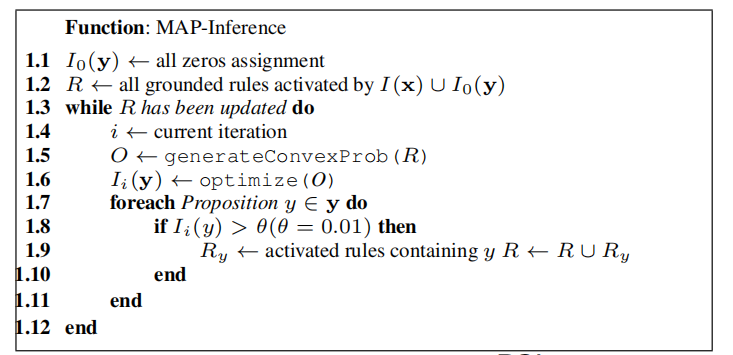
By introducing an auxiliary variable $v_a$ for each atom a, we get a value for each rule r, denoted as $v_r$. Use the inequality constraint $v_r \geq d_r(I_{i-1})$ and hard constraints to construct the SOCP with the objective function $\sum_{r\in R}\lambda_r(d_r(I))^p$.
2. Harnessing Deep Neural Networks with Logic Rules
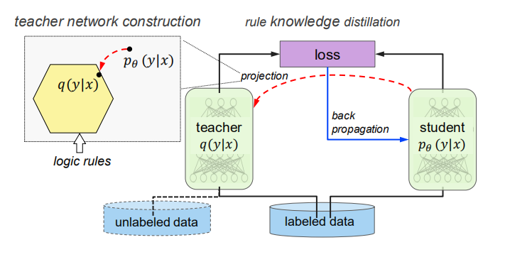
$q(y|x)$ is a projection of the true distribution $p(y|x)$ to the subspace constrained by the rules. The loss of student network is:
$$\begin{align} \boldsymbol{\theta}^{(t+1)}=\arg \min _{\theta \in \Theta} \frac{1}{N} \sum _{n=1}^{N}(1-\pi) \ell\left(\boldsymbol{y} _{n}, \boldsymbol{\sigma} _{\theta}\left(\boldsymbol{x} _{n}\right)\right) \ +\pi \ell\left(\boldsymbol{s} _{n}^{(t)}, \boldsymbol{\sigma} _{\theta}\left(\boldsymbol{x} _{n}\right)\right) \end{align}$$
where $\boldsymbol{s}_{n}^{(t)}$ is the soft prediction of q on $\boldsymbol{x}_n$, $\pi$ is the weight balancing between the task of emulating the teacher network and the task of predicting the true labels.
Compared with training a projected network and other models, the procedure has advantages:
- Better performance.
- The student network is suitable for predicting new examples in place of rule assignment.
- The two loss terms can be handled separately. Unlabeled data can be added to the second term.
How to learn the projected distribution:
$$\begin{array}{rl}
{\min \limits_{q, \xi \geq 0}} & {\mathrm{KL}\left(q(\boldsymbol{Y} | \boldsymbol{X}) | p_{\theta}(\boldsymbol{Y} | \boldsymbol{X})\right)+C \sum_{l, g_{l}} \xi_{l, g_{l}}} \\
{\text { s.t. }} & {\lambda_{l}\left(1-\mathbb{E}_{q}\left[r_{l, g_l}(\boldsymbol{X}, \boldsymbol{Y})\right]\right) \leq \xi_{l, g_{l}}} \\
{} & {g_{l}=1, \ldots, G_{l}, l=1, \ldots, L}
\end{array}$$
$r_{l,g_l}$ is the $g_l$-th grounding of the $l$-th rule. By variation, we have a closed form solution:
$$
q^{*}(\boldsymbol{Y} | \boldsymbol{X}) \propto p_{\theta}(\boldsymbol{Y} | \boldsymbol{X}) \exp \left\{ -\sum_{l, g_{l}} C \lambda_{l}\left(1-r_{l, g_{l}}(\boldsymbol{X}, \boldsymbol{Y})\right)\right\}
$$
The computation of $q$ can be tricky. Direct enumeration, dynamic programming, Gibbs sampling and joint inference are considered according to different type of logic rules. The sets of logic rules are intuitive and based on the specific task, see Applications.
- How the rule weights are derived? Hyperparameters, hard constraints are set to infinity and others 1.
3. Deep Compositional Question Answering with Neural Module Networks
Contributions:
- Neural module network - incorporating different modules into one architecture.
- Construct NMN on VQA task based on the output of a semantic parser.
- A new dataset.
Modules:
-
Attend: a conv output a heatmap indicating the region of interest.
-
Re-Attend: a mlp maps an attention to another, based on some negator or directional words.
-
Combine: two attentions stacked to one attention through a conv layer. Instances are some connectives.
-
Classify: pass original image and attention to a mlp to output classification results.
-
Measure: use to attention to predict, suitable for detection or counting.
Quetion -> Parser -> Layouts -> Activated Modules -> Prediction
A single-layer LSTM is outside NMN and also generates answers given the question without the image. Why? To introduce syntactic regularities (e.g. compensation for some loss of grammatical details from the parsing process) and semantic regularities (e.g. common knowledge like bears are usually brown not green).
4. The Neuro-Symbolic Concept Learner
github https://github.com/vacancy/NSCL-PyTorch-Release
Perception Module + Semantic Parser + Symbolic Program Executor
Visual Perception:
- pretrained Mask R-CNN for detection
- a resnet-34 extracts features from bbox and the original image respectively
- concatenate the two features to form a representation of an object
Concept Quantization
- each visual attribute corresponds to a neural operator which maps perception representations into an embedding space.
- Example: visual concepts like Cube, Sphere are learnable vectors in the embedding space of Shape.
- $\sigma\left(\left\langle\text { ShapeOf }\left(o_{i}\right), v^{\text {Cube }}\right\rangle-\gamma\right) / \tau$
- Example for computing relations of two objects: $\sigma\left(\left\langle\text { RelationOf }\left([o_{i}; o_{j}]\right), v^{\text {Left }}\right\rangle-\gamma\right) / \tau$
Semantic Parser
-
translates an question into an executable program with a hierachy of primitive operations. These operations are contained in a domain specific language(DSL).
-
The operations are kind of like the modules introduced in the last paper.
-
To make execution of operations differentiable w.r.t. visual representations, the output of an operation is a soft mask of length $\#{objects}$.
Program Execution

- Concept set ${c_i}$ is a set of all concept words appearing in questions, which is extracted using hand-coded rules. The concept words for CLEVR dataset is known. Automatic discovery of concept words is a future work.
- All decoders and encoders are bidirectional GRU network.
- Code reading….
Optimization
$$\left.\Theta_{v}, \Theta_{s} \leftarrow \arg \max _{\Theta_{v}, \Theta_{s}} \mathbb{E}_{P}\left[\operatorname{Pr}\left[A=\text { Executor(Perception }\left(S ; \Theta_{v}\right), P\right)\right]\right]$$
- $\Theta_v$ is the parameters in visual perception module (including attribute operators and concept embedding). gradient: $$\left.\nabla_{\Theta_{v}} \mathbb{E}_{P}\left[D_{\mathrm{KL}}\left(\text { Executor (Perception }\left(S ; \Theta_{v}\right), P\right) | A\right)\right]$$
- $\Theta_v$ is the parameters in sematic parsing module. REINFORCE: $r=1$ if the answer is correct otherwise 0. $$\nabla_{\Theta_{s}}=\mathbb{E}_{P}[r \cdot \log \operatorname{Pr}[P=\text { SemanticParse }\left(Q ; \Theta_{s}\right)]]$$. It is approximated via Monte Carlo.
Experiments
How well the visual concepts are learned?
- Use the perception module only to do classification, near perfect performance.
- Use “How Many” question to evalute the performance.
What’s Program Annotation?
How well the semantic parsers are learned?
- Evaluate the accuracy of programs by executing them on the ground-truth annotations of objects.
Curriculum learning: split the training samples into 4 stages with incremental complexity of scenes and questions and train the model with the dataset stage by stage.
Advantages:
- No need for class labels for objects.
- Strong ability of generalization
5.Neural Aspect and Opinion Term Extraction with Mined Rules as Weak Supervision
$D_l$ labeled data,$D_a$ unlabeled data
-
Mine a set of aspect extraction rules $R_a$ and a set of opinion extraction rules $R_o$
-
Extract terms for reviews in $D_a$ with mined rules, which can be used as a weakly labeled dataset $D_{a’}$
-
Train a neural network based on $D_l$ and $D_{a’} $
Dependency Relation Extraction: (rel, $w_g$, $w_d$) denotes the dependency exists between $w_d$the governor and $w_d$ the dependent.

Generate rule candidates based on a training set and filter the rule candidates based on a val set.
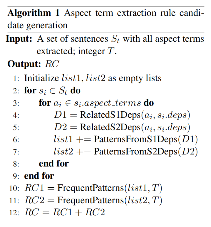
Explanation of the pseudo-code:
-
$s_i.deps$ is the list of the dependency relations obtained by parsing. $list1$ and $list2$ contain the possible term extraction patterns.
-
PatternsFromS1Deps can generate the following patterns from $(rel, w_g, w_d)$: $(rel, w_g, ps(w_d)^*)$, $(rel, POS(w_g), ps(w_d)^*)$, $(rel, O, ps(w_d)^*)$, where $O$ is a predefined set of opinion words. For aspect words, only nouns and verbs and considered.
-
PatternsFromS2Deps generate patterns based on pairs of patterns returned by PatternFromS1Deps, and outputs all possible pattern pairs if there is a shared word in the dependency relation pair. (??? why output pair???)
|
|
- FrequentPatterns calculates the frequency of each rule candidate and delete the patterns appearing in the dataset less than $T$ times.
Later homework: Dependency Parsing…
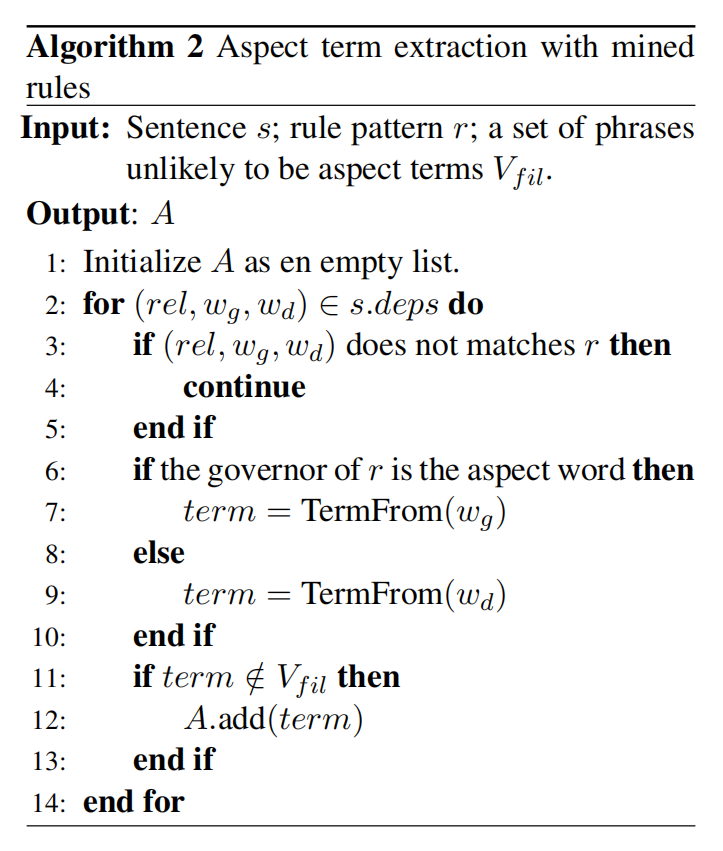
TermFrom return the word $w$ if $w$ is a verb, and when $w$ is a noun it returns the noun phrase formed by the consecutive sequence of noun words including noun. $V_{fil}$ is a set of words that are unlikely to be aspect terms.
Models and Training:
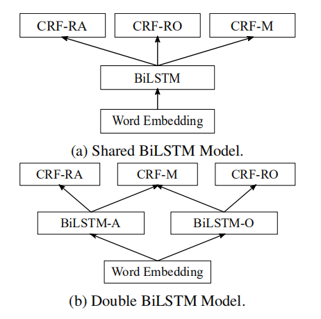
A and O are for aspect and opinion term extraction, M for manual label prediction. Three tasks are trained in 2 ways with two models shown in the figure. 1) train on the three tasks $t_a,\ t_o$ and $t_m$ alternately 2) pretrain on $t_a$ and $t_o$, then train on $t_m$. The evaluation metric is F1-score.
For pseudo-labeled dataset, two copies of each sequence are fed to the model because a word can be both an aspect term and an opinion term due to inaccurate rules. There is no such need for $D_l$.
6. DL2: Training and Querying Neural Networks with Logic
Flaws of two methods with logic reasoning mentioned above:
-
PSL: incompatible with gradient-based optimization
-
rule knowledge distillation: a) only constraints w.r.t. $X$ and $Y$ can be used and b) non-linear constraints w.r.t $Y$ leads to violation of convexity.
Constrained Neural Network
Define: A term $t$ can be input $\mathbf x$ or network weights $\theta$ or their (almost) differentiable functions.
Comparison constraint: $t< t'$, $t = t'$, $t\not = t'$, $t\leq t'$
Constraint $\varphi$ is made up of comparison constraints with $\wedge$ , $\lor$, $\neg$
Translation into loss:
$$
\begin{aligned}
\mathcal{L}\left(t \leq t^{\prime}\right)&:=\max \left(t-t^{\prime}, 0\right)\\
\mathcal{L}\left(t \neq t^{\prime}\right)&:=\xi \cdot\left[t=t^{\prime}\right]\\
{\mathcal{L}\left(\varphi^{\prime} \wedge \varphi^{\prime \prime}\right)} &:={\mathcal{L}\left(\varphi^{\prime}\right)+\mathcal{L}\left(\varphi^{\prime \prime}\right)} \\
{\mathcal{L}\left(\varphi^{\prime} \vee \varphi^{\prime \prime}\right)} &:={\mathcal{L}\left(\varphi^{\prime}\right) \cdot \mathcal{L}\left(\varphi^{\prime \prime}\right)}
\end{aligned}
$$
Negation of a constraint can be rewritten into an equivalent constraint before translation into a loss.
Theorem 1: Non-negative loss $L(\varphi) = 0$ iff $\varphi$ is satisfied.
Training loss: $$\underset{\theta}{\arg \max } \operatorname{Pr}_ {\boldsymbol{x} \sim \mathcal{D}} [\forall \boldsymbol{z} \in \mathbb{A}, \varphi(\boldsymbol{x}, \boldsymbol{z}, \theta)]$$
can be transformed to
$$ \underset{\theta}{\arg \max } \operatorname{Pr}_ {\boldsymbol{x} \sim \mathcal{D}}\left[\varphi\left(\boldsymbol{x}, \boldsymbol{z}^{*}(\boldsymbol{x}, \theta), \theta\right)\right] \
z^{*}(\boldsymbol{x}, \theta)=\underset{\boldsymbol{z} \in \mathbb{A}}{\arg \max }[\neg \varphi(\boldsymbol{x}, \boldsymbol{z}, \theta)] $$
which follows the pattern of adversarial training: find the adversary violating the constraint and minimize the risk corresponding to the adversary.
By theorem 1, we have approximation
$$
\boldsymbol{z} ^{*}(\boldsymbol{x}, \theta)=\underset{\boldsymbol{z} \in \mathbb{A}}{\arg \min } \mathcal{L}(\neg \varphi)(\boldsymbol{x}, \boldsymbol{z}, \theta)\
\underset{\theta}{\arg \min } \underset{\boldsymbol{x} \sim \mathcal{T}}{\mathbb{E}}\left[\mathcal{L}(\varphi)\left(\boldsymbol{x}, \boldsymbol{z} ^{*}(\boldsymbol{x}, \theta), \theta\right)\right]
$$
where $\boldsymbol x\sim \mathcal T$ means drawing x uniformly from dataset T to approximate distribution $\mathcal D$.
For constraints like $|\boldsymbol x - \boldsymbol z | < \epsilon$, we use them as convex sets for projected gradient descent rather than translate them into losses.
Quering Networks
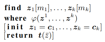
$\mathbf{find}$ defines a number of variables with given shape. The last two clauses can be omitted. When $\mathbf{return}$ clause is missing, the variables in $\mathbf{find}$ clause will be returned.
Example:
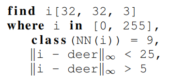
$\mathbf{class}$ NN(i) = y is equivalent to $\bigwedge_{i=1, i \neq \mathrm{y}}^{k} p(x)_{i}<p(x)_{y}$. $\mathbf{in}$ for box constraints imposed on all elements in i(syntactic sugar). The constraint with infinity norm will be translated into equivalent version $\bigwedge_j |i_j|<\epsilon$.
DL2 translates these constraints into losses and find the optimizer with L-BFGS-B as the solution. If the solution is not found after a certain time, we restart L-BFGS-B and reinitialize the variables using MCMC sampling.
Training
For all experiments, a cross-entropy term is added to the loss.
-
Semi-Supervised Learning:
Train network with cross-entropy loss on labeled data, and the DL2 encoding of constraints like $\left(p_{\text {people}}<\epsilon \vee p_{\text {people}}>1-\epsilon\right)$ $\wedge \ldots$ $\wedge\left(p_{\text {trees}}<\epsilon \vee p_{\text {trees}}>1-\epsilon\right)$ to force predictions into groups on unlabeled data.
-
Unsupervised Learning:
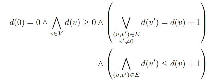
To train a MLP to predict the minimum distance between two nodes on a given graph $G = (V, E)$, we can use a logical constraint like rules in dynamic program:
-
Supervised Learning
Training neural networks meeting some sort of smoothness is desirable recently. Like Lipschitz: $$\left|\operatorname{logit} _{\theta}(\boldsymbol{x})-\operatorname{logit} _{\theta}\left(\boldsymbol{x}^{\prime}\right)\right| _{2}<L\left|\boldsymbol{x}-\boldsymbol{x}^{\prime}\right| _{2}$$
More generally, thanks to introduction of $z$, global constraints of Lipschitz can be:
$$ \left|\operatorname{logit} _{\theta}(\boldsymbol{z})-\operatorname{logit} _{\theta}\left(\boldsymbol{z}^{\prime}\right)\right| _{2}<L\left|\boldsymbol{z}-\boldsymbol{z}^{\prime}\right| _{2},\ \forall \boldsymbol{z} \in B _{\epsilon}(\boldsymbol{x}) \cap[0,1]^{d}, \boldsymbol{z}^{\prime} \in B _{\epsilon}\left(\boldsymbol{x}^{\prime}\right) \cap[0,1]^{d} $$