Evolvement of Recommendation System Algorithms
Contents
Machine Learning Models
CF - Collaborative Filtering
To recommend new items to a user u, we can use the existing scores that u has already scored. At the same time, the similarity between two items can be evaluated by the review scores from all users. According to the feedback of items that the user u has already evaluated, we can estimate the score of the product p:
$$ R_{u,p} = \sum _{h\in H} w_{ph}\cdot R_{uh} $$
$$ w_{ph} = \frac{\sum _{v \in U_p \cap U_h} R_{vp} R_{vh}}{\sqrt{\sum _{v \in U_p} R_{vp}^2} \sqrt{\sum _{v \in U_h} R_{vh}^2}} $$
where $H$ is the set of products u has scored and $U_p$, $U_h$ are the users who have scored the product p and h respectively. Here the similarity is defined as cosine similarity, while pearson similarity is more common in information retrieval.
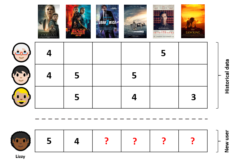
FM Factorization Machine
It is an improved version of logistic regression, which uses the product of embedding vectors $ \mathbf {w} _i^T \cdot \mathbf{w} _j $ to substitute the interaction term $w _{ij}$. This method reduces the parameters from $n^2$ to $nk$, where $k$ is the embedding dimension.
FFM
The concept of field is introduced based on FM. It is equivalent to split an original sparse features into $f$ sparse features (use $f$ different embeddings for the same sparse feature), where $f$ is the number of fields. For example, feature i and feature j belong to the field a, and feature k belongs to the field b. For the interaction term of feature i & j, it is $\mathbf {w} _{ia} ^T \mathbf {w} _{ja}$, while the interaction term of feature i & k is $\mathbf{w} _{ib}^T \mathbf{w} _{ka}$. The number of parameters is $knf$.
GBDT+LR
For each subtree of GBDT, each input x will be assigned to a certain leaf node. Set this leaf node to 1, and set other leaf nodes to 0, and then we get a representation of this subtree, which looks like a binary vector. The feature vectors of the subtrees are concatenated to get a high-dimensional sparse vector, which is then passed to LR for CTR prediction.
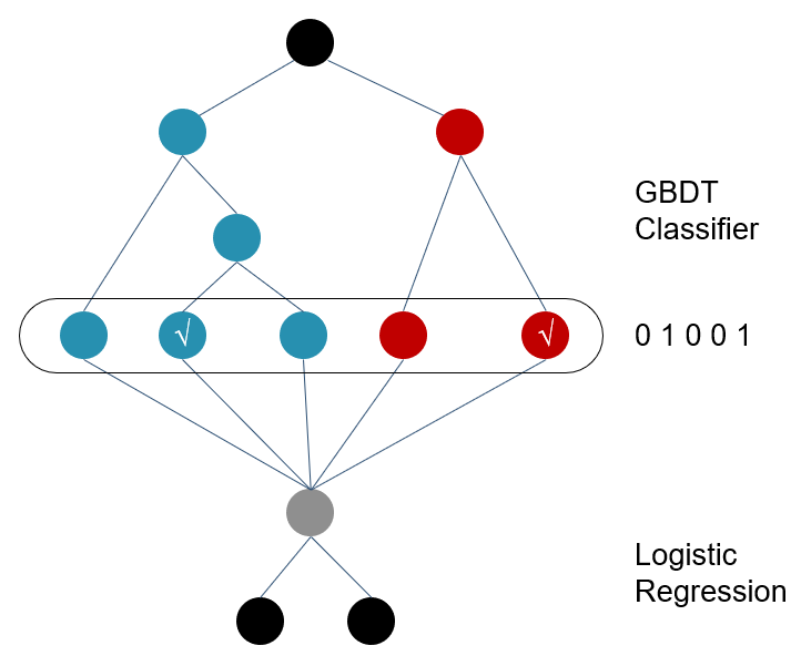
Advantages of regression trees:
- High-order interaction features can be learned, and this order can be as high as the depth of the subtree.
Disadvantages of regression trees:
- A large amount of accurate numerical information is lost
- It is prone to overfitting.
- The training time of GBDT is too long.
LS-PLM
This methods incorporates the idea of clustering (Mixture Model) into logistic regression. Separate items into $m$ subclasses, train $m$ different LR models for these subclasses and train a softmax regression model to predict the probability that the input $x$ belongs to each subclass. $$ f(x) = \sum_{i=1}^{m} \pi_i(x) \eta_i(x) = \sum_{i=1}^m \frac{e^{\mu_ix}}{\sum_{j=1}^m e^{\mu_jx}}\cdot \frac{1}{1+e^{-w_ix}} $$ Advantage:
- Nonlinearity brings better model capacity
- Grouped L2 norm is added to improve generalization
Deep Learning Model
AutoRec
Let $V$ be the scoring matrix. Here an auto-encoder is trained to reconstruct the scoring matrix. The hidden layer can be interpreted as a set of user embeddings and item embeddings.
$$ min \sum_{i=1}^n \Vert V_{i}-h(V_i;\theta) \Vert^2 + \frac{\lambda}{2}(\Vert W \Vert^2 + \Vert V\Vert^2) $$
where $W$ is parameters of MLP.
Neural CF
Embedding layer is used to extract representation vectors for users and items. Instead of inner product, Neural CF feeds the vector of user u and item p to an MLP to predict CTR. It is because MLP is better at feature interaction than a simple operation like inner product. Besides, we can do element-wise product of the u vector and p vector, insert the product vector to the hidden layer can lead to more complicated feature interaction.
PNN
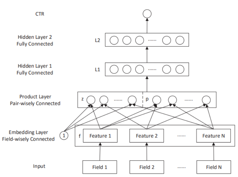
The first layer is an embedding layer, which converts the sparse categorical features into dense embeddings. Then there are two ways of feature interactions in the product layer. They are inner product and outer product, namely $f _i f _j ^T$. However, the output of outer product must be a matrix rather than a scalar like inner product. So a dimension reduction is applied to outer production:
$$ p = \sum_{i=1}^{M}\sum_{j=1}^{M}f_if_j^T = f_{\Sigma} f_\Sigma^T, \ \ \ f_\Sigma = \sum f_i $$ This operation can be interpreted as a kind of average pooling.
Then two parallel fully-connected layers are used to map output from inner product and output from outer product into two vectors with the same dimension. And after that, these two vectors get concatenated and fed into the top MLPs.
Attention: in practice, average pooling should be used only within the same feature filed, because embedding vectors from different fields don’t share the same linear space.
Wide & Deep
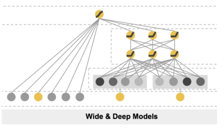
W&D model is able to merge different types of features. Numeric features can be directly input into fully-connected layer, while categorical features will first go through the embedding layer. Numeric features and embeddings are stacked together and fed into the Deep module on the right. The Wide module on the left handles the feature interaction via
$$ \phi_k(x) = \prod_{i=1}^d x_i^{c_{ik}},\ c_{ik}=1,\ 0$$
where $c_{ki}$ is a boolean variable that is 1 if the i-th feature is part of the k-th transformation $\phi _k$, and 0 otherwise. Then Wide concatenate all transformations to a vector $\phi(\mathbf x)$. The final output is formulated as:
$$ P(Y=1 | \mathbf{x})=\sigma\left(\mathbf{w}_{\text {wide}}^{T}[\mathbf{x}, \phi(\mathbf{x})]+\mathbf{w} _{\text {deep}}^{T} a^{\left(l _{f}\right)}+b\right) $$
Why Wide&Deep is successful:
- The combination of memorization from Wide module and generalization from Deep module.
DeepFM
Due to the fact that the interaction transformations of Wide part are manually designed, FM is put forward to replace the Wide module. Here comes DeepFM.
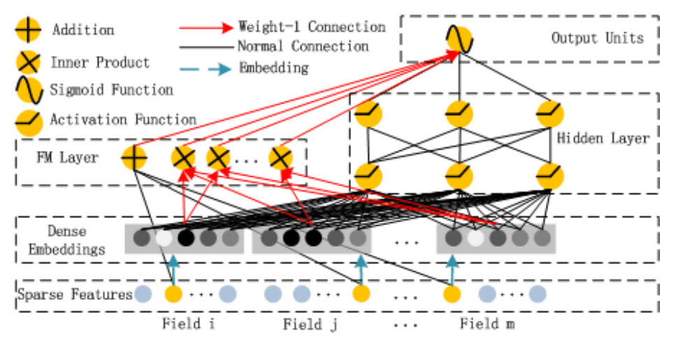
Then the output of Wide part becomes:
$$ y_{FM} = \langle w, x \rangle + \sum_{i=1}^n\sum_{j=i+1}^n \langle V_i, V_j \rangle x_i x_j $$
DIN
DIN is an application of attention mechanism in recommendation systems. It is inspired by the idea that some features play much more important roles in CTR prediction than the others. For example, users who have bought a mouse are more likely to click on an ad about keyboards. Attention is useful for automatically allocating importance weights to different features.
$$ V_u = \sum_{i=1}^N g(V_i, V_a) V_i$$
where $V_u$ is the embedding for user u and $V_a$ is the embedding for item a. $V_i$ is the embedding of user u's i-th action. The attention score is attained from a MLP with the input of $[V _i, V _i - V _a, V _a]$.