All About AUC

Definition

A formal definition of AUC is: $$AUC=P(f(x)>f(y)),\ x\sim \mathcal D _{+}, y\sim \mathcal D _{-}$$

where $\mathcal D _+$ is the set of positive samples, and $\mathcal D _-$ is the set of negative samples. Therefore, the metric of AUC can be interpreted as “the probability that a positive sample is wrongly ranked ahead of a negative sample”. AUC can naturally measure the performance of a binary classification model and is thus widely used in evaluating recommendation systems. Also, its resistance against class imbalance is helpful when handling skewed data.

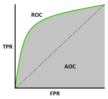
While in machine learning related classes, we are often told that AUC stands for the Area Under the Curve, where the curve refers to the ROC Curve. First, let me introduce the ROC Curve - the curve showing the relation between True Positive Rate (TPR) and False Positive Rate (FPR):

$$ TPR = \frac{TP}{TP+FN} $$

$$ FPR = \frac{FP}{FP+TN} $$

Given any threshold $t$ in $[0,1]$, we determine whether a sample is predicted as positive by checking if $f(x) > t$, and then we can derive the corresponding $TPR(t)$ and $FPR(t)$ as functions of $t$. With this parameter $t$, we can easily draw the ROC Curve.

Here is a mathematical proof about the relation between the probability definition and the area definition of AUC:

Let $s_+$ and $s_-$ be the score of a random positive/negative sample. Consider the probability that the $s_-$ lies between $[t, t+\Delta t]$: $$\begin{aligned} & P\left(t \leq s_{-}<t+\Delta t\right) \\
=& P\left(s_{-}>t\right)-P\left(s_{-}>t+\Delta t\right) \\
=& \frac{N_{-}(t)-N_{-}(t+\Delta t)}{N_{-}} \\
=& FPR(t)-FPR(t+\Delta t)=-\Delta FPR(t) \end{aligned}$$ Suppose $\Delta t$ is sufficiently small, then the conditional probability that $s_+$ is bigger than $s_-$ is $$ \begin{aligned} &P\left(s_{+}>s_{-} \mid t \leq s_{-}<t+\Delta t\right) \\
&\approx P\left(s_{+}>t\right)=\frac{\text{# of pos samples predicted as pos}}{\text{# of pos samples}}\\
&=\frac{TP(t)}{P}=TPR(t) \end{aligned} $$ Then, $$\begin{aligned} & P\left(s_{+}>s_{-}\right) \\
=& \sum_t P\left (t \leq s_{-}<t+\Delta t\right) P\left(s_{+}>s_{-} \mid t \leq s_{-}<t+\Delta t\right) \\
=&-\sum_{t} TPR(t) \Delta FPR(t) \\
=&-\int_{t=-\infty}^{\infty} TPR(t) d FPR(t) \\
=& \int_{t=\infty}^{-\infty} TPR(t) d FPR(t) \end{aligned}$$

• Why do we interchange the limits in the last step? It’s because $FPR(t)$ decreases when $t$ goes up. We want the x-axis to be increasing and thus $t$ must be decreasing.

Therefore, the two definitions are completely equivalent. Though, the area definition is more intuitive and more often talked about.

Calculation

Based on the two types of definition, how do we use Python or SQL to calculate the AUC if we are given the labels and predicted scores of samples?

1. Calculation by Area

Based on the area definition, we can divide the x-axis into lots of small intervals and use trapeziums to approximate the area.

 1
 2
 3
 4
 5
 6
 7
 8
 9
10
11
12
13
14
15
16
17
18
19
20
21
22
23
24
25
26
27
28
29
30
31
32
33
34
35
36

def calcAUC_by_area(labels,probs):
    ###initialize
    P = 0
    N = 0
    for i in labels:
        if (i == 1):
            P += 1
        else:
            N += 1
    TP = 0
    FP = 0
    TPR_last = 0
    FPR_last = 0
    AUC = 0
    pair = zip(probs, labels)
    pair = sorted(pair, key=lambda x:x[0], reverse=True)
    i = 0
    while i < len(pair):
        if (pair[i][1] == 1):
            TP += 1
        else:
            FP += 1
        ### maybe have the same probs
        while (i + 1 < len(pair) and pair[i][0] == pair[i+1][0]):
            i += 1
            if (pair[i][1] == 1):
                TP += 1
            else:
                FP += 1
        TPR = TP / P
        FPR = FP / N
        AUC += 0.5 * (TPR + TPR_last) * (FPR - FPR_last)    ## area equation for trapezium
        TPR_last = TPR
        FPR_last = FPR
        i += 1
    return AUC

2. Calculation by Reverse Pairs

How do you estimate the probability that a positive sample ranks higher than a negative sample? A very intuitive solution may be

$$ \frac{\text{# pair of samples such that $f(a) > f(b)$ and $label(a) > label(b)$}}{\text{# pair of samples}} $$

And it can be proved that this is actually a maximum likelihood estimator. Therefore, the algorithm is like:

 1
 2
 3
 4
 5
 6
 7
 8
 9
10
11
12
13
14
15
16
17
18
19
20

def calcAUC_by_prob(labels, probs):
    N = 0
    P = 0
    neg_prob = []
    pos_prob = []
    for idx, label in enumerate(labels):
        if (label == 1):
            P += 1
            pos_prob.append(probs[idx])
        else:
            N += 1
            neg_prob.append(probs[idx])
    number = 0
    for pos in pos_prob:
        for neg in neg_prob:
            if (pos > neg):
                number += 1
            elif (pos == neg):
                number += 0.5
    return number / (N * P)

However, this implementation is not satisfactory due to its two layers of for-loops, which accounts for $O(n^2)$ time complexity.

Actually, we can sort the samples with regard to its prediction value in ascending order, and then find the number of reverse pairs (namely $i < j$ $\land$ $nums[i] > nums[j]$). Therefore, a MergeSort based algorithm can reduce the time complexity to $O(n\log n)$.

Another idea is from the reference blog. Let’s consider a random positive sample. Assume that it is ranked j-th among all positive samples. Then there are $j-1$ positive samples before it. And assume that its ranking among all samples is $r_j$. Then there are $r_j - j$ negative samples before it. So, the probability that another random negative sample lies before this positive sample is $(r_j - j)/N_-$, where $N_-$ is the number of negative samples. Given this, let’s average the probability over all $j$:

$$ AUC = \frac{1}{N_{+}} \sum_{j=1}^{N_{+}}\left(r_{j}-j\right) / N_{-}=\frac{\sum_{j=1}^{N_{+}} r_{j}-N_{+}\left(N_{+}+1\right) / 2}{N_{+} N_{-}}$$

The implementation becomes:

 1
 2
 3
 4
 5
 6
 7
 8
 9
10
11
12
13
14
15

def calAUC(labels,prob):
    f = list(zip(prob,labels))
    rank = [values2 for values1,values2 in sorted(f,key=lambda x:x[0])]
    rankList = [i+1 for i in range(len(rank)) if rank[i]==1]
    posNum = 0
    negNum = 0
    for i in range(len(labels)):
        if(labels[i]==1):
            posNum+=1
        else:
            negNum+=1
    auc = 0
    auc = (sum(rankList)- (posNum*(posNum+1))/2)/(posNum*negNum)
    print(auc)
    return auc

There is another way of implementing this calculation in SQL:

 1
 2
 3
 4
 5
 6
 7
 8
 9
10
11
12
13
14
15

select
  (ry - 0.5*n1*(n1+1))/n0/n1 as auc
from(
  select
    sum(if(y=0, 1, 0)) as n0,
    sum(if(y=1, 1, 0)) as n1,
    sum(if(y=1, r, 0)) as ry
  from(
    select y, row_number() over(order by score asc) as r
    from(
      select y, score
      from some.table
    )A
  )B
)C

Reference

[1] https://tracholar.github.io/machine-learning/2018/01/26/auc.html

[2] https://developers.google.com/machine-learning/crash-course/classification/roc-and-auc